Climate Change and Economy
European satellite data of the Copernicus space program:
High humidity and low solar radiation (Winkler Index) and its possible impact on Chilean vineyards.
Processing of satellite statistical information with "R" programming language
Author: Fernando M. Roque R.
Facebook: https://www.facebook.com/stdepiphron
Twitter: https://twitter.com/epiphron1
Email: qestadinfo@gmail.com
1
.Summary
The use of satellite data from the European Copernicus program can be useful for the analysis of climate adaptation in areas where there is no earth sensor infrastructure. For example the wine areas of Chile and the dry corridor in Central America.
To carry out these analyses, the Soil Water Index product (Copernicus Water Index or soil moisture) was used. The address of this product is here: https://land.copernicus.eu/global/products/swi
A case study that proves the validity of satellite data is the drought that has affected California and Australia since 2012 and is recorded by the ground and image sensors of the US drought monitor (https: //droughtmonitor.unl.edu /) for California and the Australia Bureau of Meteorology (http://www.bom.gov.au/climate/)
Image 1.1 |


|
|
|

|
|
|


Economically California's agricultural production mainly of Valencia oranges, corn, broccoli, and asparagus was affected.
In the case of Central America, the drought detected by the satellite data is confirmed by the disappearance of a Laguna in the Dry Corridor of Guatemala published by an article by National Geographic (https://news.nationalgeographic.com/2017/05/lake -atescatempa-guatemala-drought-el-nino-video/ ). In addition to the economic crisis of coffee and migration to the United States due to the lack of rain in coffee growing areas. Huffington Post published an article about this situation.
Link: https://www.huffingtonpost.com/entry/climate-change-coffee-guatemala_us_589dd223e4b094a129ea4ea2
Crisis of the drought in Guatemala, Central America detected by the Soil Water Index for three regions during the years 2013 to 2016.
Image 1.7
The situation in Chile. The wine regions of Chile studied have similar weather seasons in these months:

In Chile there are four stations on these dates:
a) Summer: December 21 (solstice) to March 20 (equinox).
b) Autumn: March 20 to June 21 (solstice)
c) Winter: June 21 to September 23 (equinox).
d) Spring: September 23 to December 21 (solstice)
The period with the highest rainfall is from May to September. The theoretical behavior of rain and dry season in Chile is given by this graph of the Valparaíso and Rancagua region:
|

The factor that most affects the growth and quality of the vine and grapes are the days of solar exposure between the months of October and April. This factor is the Winkler index. The vine must have a high accumulation of days with solar radiation so that the Winkler index is high and the quality is better.
The information from Copernicus shows a high soil moisture variability for the Chilean wine regions during the most important months of the summer between October and April. High humidity in the soil could indicate that there were several cloudy days in those days and affected the Winkler index.
The graph shows that as of March 2016, the soil moisture during the growth of the vine has grown. Probably affecting the Wrinkler index. Image 1.9 |

The standard deviation of the regions studied shows a large amplitude of the data, especially in the regions of and during the summer season. This indicates that the regions should be segmented to see which areas are most affected by climate variability and which are more resistant.
|

The processing of the satellite data was done using the programming language "R". The program reads the desired coordinates of desired latitude and longitude of the Copernicus NetCDF file. From here, a comma-separated format file (.CSV) is written and loaded into a MYSQL database.
The statistical analysis of data is carried out with programming functions and graphics of the "R" language. The explanation of the code and the source program are in section x.y). They are also placed in this direction of GITHUB.
2) CHILE'S WINE ZONES: CLASSIFICATION BY TEMPERATURE AND RAINS. RELATIONSHIP BETWEEN QUALITY AND CLIMATIC PARAMETERS. INDEX OF WINKLER.
2.1) REGIONS, CLIMATES, AND VARIETIES
In Chile there are four stations on these dates:
a) Summer: December 21 (solstice) to March 20 (equinox).
b) Autumn: March 20 to June 21 (solstice)
c) Winter: June 21 to September 23 (equinox).
d) Spring: September 23 to December 21 (solstice)
The rainiest months are those of winter. June to September.
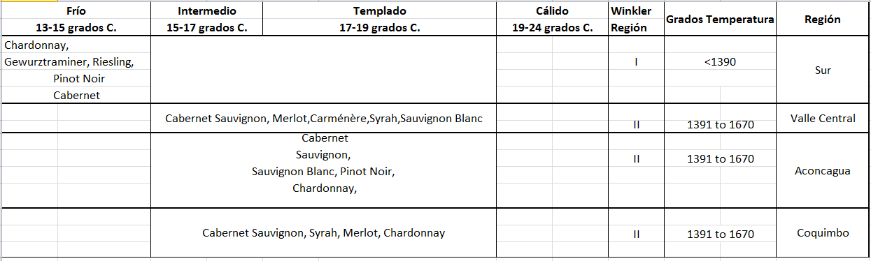
Región | Zonas | Clima | Variedad |
Coquimbo | Valles de Elquí y Limarí | Little precipitation and coastal fog. | Cabernet Sauvignon, Syrah, Merlot, Chardonnay |
Aconcagua | Aconcagua, Casa Blanca, San Antonio | Moderate temperature due to maritime influence. Mediterranean climate, semi-desert. The Humboldt current from the Arctic brings cold temperatures to the coast. Example: Valparaíso. January 18 degrees C. July 13 degrees C. Drip irrigation due to low rainfall. It receives high levels of solar radiation, an important factor for the vineyards. Source: http://aconcagua.wine/clima/ | Cabernet Sauvignon, Sauvignon Blanc, Pinot Noir, Chardonnay, |
Valle Central | Maipo, Cachapoal, Colchagua, Curicó, Maule | Temperate-warm, dry summers and with high temperatures, frosts in spring. High levels of solar radiation. Heavy rains in winter. Mediterranean climate with temperate and rainy winters and dry summers. | Cabernet Sauvignon, Merlot, Carménère, Syrah, Sauvignon Blanc |
Región Sur | Itata, Bío Bío, Malleco |
| Moscatel de Gewurztraminer, Riesling, Pinot Noir |
2.2) QUALITY AND CLIMATIC PARAMETERS
The Winkler indicator is a parameter used to classify wine regions and can be used to measure the impact that Climate Change will have on wine production and flavors. This indicator measures the accumulation of heat from the daily average temperature of 10 degrees Celsius during the months of vine growth. In the southern hemisphere, these months are from October to April. According to the accumulation of heat, so will be the variety that can be harvested in that region.
Cold 13-15 degrees/Medium 15-17 degrees/Tempered 17-19/degrees Warm 19-24/degrees/TemperatureDegrees/Region |
3) STUDY OF SOIL MOISTURE WITH SATELLITE DATA OF COPERNICUS FOR FOUR REGIONS OF CHILE BETWEEN THE YEARS 2009 TO 2019.
3.1) ANALYSIS FOR VICUÑA, PROVINCE OF ELQUIA, COQUIMBO REGION
The summers are dry, hot, arid and clear. The winters are dry and clear. What favors solar radiation and improves the Winkler indicator, since from October to April is when you have high solar exposure. Source: https://es.weatherspark.com/y/26539/Clima-promedio-en-Vicu%C3%B1a-Chile-durante-todoel-a%C3%B1o
These are the "normal" conditions until a few years ago. However, this balance has been broken with irregular rainfall in winter since 2009 and with precipitation in summer, which was not typical of this region. Source: http://www.uchile.cl/noticias/144130/las-lluvias-a-lo-largo-y-ancho-de-chile-explicadas-en-10-datos and https://www.biobiochile.cl/news/national/chile/2019/02/05/ lluvia-del-norte-y-calor-record-en-el-sur-como-se-viene-el-clima-en-chile-para-los- next-days.shtml
Data and reference chart for annual precipitation.
|
https://es.weatherspark.com/y/26539/Clima-promedio-en-Vicu%C3%B1a-Chile-durante-todo-el-a%C3%B1o |

Region of Coquimbo studied by European satellite Copernicus using soil moisture indicator, Soil Water Index.
Image 3.1.2 |

Results of Copernicus satellite data
Several comparative graphs are presented for different seasons of the climate, growth of the vine and indicators accumulated for each climatological station. Graphics:
- Times of the year: rainy season (June to September), dry season (December to March) and vine growth (October to April). The latter is important because of the Winkler indicator, which depends on the amount of solar radiation the plant receives in those months.
-Accumulated Soil Water Index for each climate station described above. This will give us a parameter of what the general situation is at the end of each season, compared to the years of study that are from 2009 to 2019.
- The standard deviation for each of the seasons of the soil moisture indicator (Soil Water Index). These data give an idea of the variability of humidity that may exist in the region studied. A high standard deviation indicates that the humidity is not uniform and that segmentation of the area must be carried out in order to find the most regular humidity throughout the year. For wine cultivation, which needs stable conditions in each season of the climate and in the growing areas, it is critical that these variables be as stable as possible.
Image 3.1.3 Soil Water Index Soil Moisture. Rainy Season June to September |

In the graph, you can see a wide variability of humidity for the months of the rainy season, from June to September. The years 2009 and 2010 were humid, but in 2011 the winter was dry. It recovered in 2012 to fall approximately in half in 2013. The years 2014 and 2015 had high humidity. However, in 2016, winter again became scarce in the rainy season. The years 2017 and 2018 were humid, especially in 2018. This variability in rainfall levels could affect the planting of the vine that expects to have stable conditions in each season.
Image 3.1.2 Soil Water Index Soil Moisture. Dry Season December to March |
The summers of 2014 and 2015 were quite humid compared to 2013 and 2012. From 2016 to 2018 the soil moisture in summer has been relatively equal. In 2019, the humidity index is almost at the 2015 levels. In 2009 it was the last year with humidity levels. The irregular situation began in 2010 with high humidity levels, reaching the maximum in 2014, 2015 and 2019. The summer is from December to April, which is supposed to be when more solar radiation is needed for the growth of the vine. These high levels of humidity may have created cloudy in the sky, affecting the sunlight. |
Image 3.1.3 Soil Water Index Soil Moisture. Growth of the vine. October to April |


The years 2013, 14, 15 and 19 had high levels of humidity for the period of growth of the vine and that affects the Wrinkler index. The humidity could indicate that during these months of these years there were clouds that affected the solar radiation. The years 2016,17 and 18 had less humidity compared with those described above. The monitoring should be done in the growth of the vine for the year 2019 since as explained, it had a return to the situation of high humidity levels.
Image 3.1.4 Accumulated soil moisture for Rainy Season 2009-2018 |

Image 3.1.5 Accumulated soil moisture for Dry Season 2009-2018 |

Image 3.1.6 Accumulated Soil Water Index Soil Moisture. Growth of the vine. October to April |

3.2) ANALYSIS FOR REGIONS OF VALPARAÍSO (V) AND RANCAGUA (VI)
REGION STUDYED BY SATELLITE COPERNICUS, VALPARAÍSO (REGION V), SANTIAGO, RANCAGUA (REGION VI).
Image 3.2.1 | Image 3.2.2 |


In Valparaíso, the rainy season is four months, between the months of May to September. The dry season is 7 months from September to April.
Source: https://es.weatherspark.com/y/25811/Clima-promedio-en-Valpara%C3%ADso-Chile-durante-todo-el-a%C3%B1o Image 3.2.3 |
In Rancagua the months of precipitation are from April to October. The dry season is from mid-October to the end of March. This region coincides with the growth of the vine. In theory, its dry season is associated with a high value of the Winkler index.
|
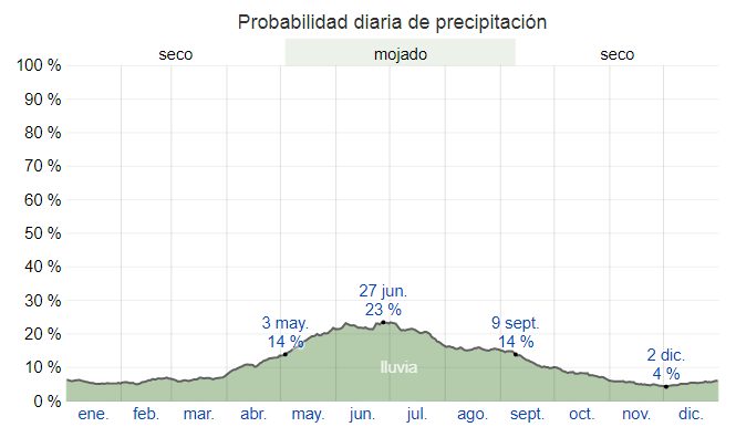
Image 3.2.5 |

.
Image 3.2.6 |

Image 3.2.7 |
Image 3.2.8 |

3.3) ANALYSIS FOR MAULE REGION
Maule region studied by Copernicus satellite.
Image 3.3.1 | Image 3.3.2 |


The rainy season in Maule is from May to September. The dry season coincides with the growth of the vine, which is from October to April. Source: https://es.weatherspark.com/y/25795/Clima-promedio-en-Talca-Chile-durante-todoel-a%C3%B1o
Source: https://es.weatherspark.com/y/25795/Clima-promedio-en-Talca-Chile-durante-todo-el-a%C3%B1o Image 3.3.3 Daily precipitation probability |

Image 3.3.4 |

Image 3.3.5 |

Image 3.3.6 |
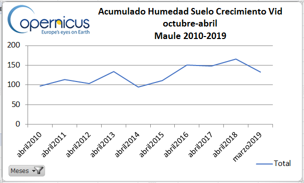
Image 3.3.7 |

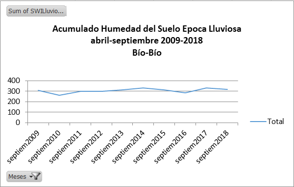
3.4) ANALYSIS FOR BÍO BÍO REGION
Bío Bío region studied by Copernicus satellite.
Image 3.4.1 | Image 3.4.2 |


The rainy season in Bío Bío is from May to September. The dry season coincides with the growth of the vine, which is from October to April. Source: https://es.weatherspark.com/y/25795/Clima-promedio-en-Talca-Chile-durante-todoel-a%C3%B1o
Source: https://es.weatherspark.com/y/25795/Clima-promedio-en-Talca-Chile-durante-todo-el-a%C3%B1o Image 3.4.3 Daily precipitation probability |
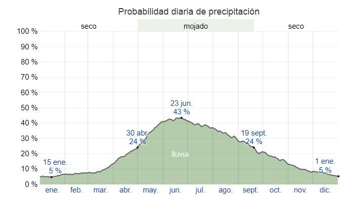
Image 3.4.4 |

Image 3.4.5 Soil Water Index Soil Moisture. Growth of the vine. October to April |

Image 3.4.6 |

|
Image 3.4.7 |

4) USE OF STANDARD DEFLECTION TO OBTAIN THE UPPER AND LOWER LIMITS OF SOIL MOISTURE FOR THE REGIONS OF CHILE STUDIED
The average and the standard deviation are combined to determine the amplitude of the data obtained for each of the regions described above. A wide distance between the average and the upper and lower limits indicates that the region consists of several segments that must be studied separately. So you can have segments where soil moisture is stable during dry and rainy seasons. On the contrary, a large distance indicates a wide dispersion and that the region consists of several different segments that must be separated for study.
4.1) Coquimbo REGION
A variable situation like this indicates that the weather conditions are different even within the same region and area of cultivation. The region of Coquimbo can be divided into several sub-regions and find the best ones that meet the ideal scenario of scarce and moderate rain in the rainy season and abundant sunlight in the dry season, which should contribute to the Winkler parameter.
For the Coquimbo region, the region studied by satellite from 2009 until 2019 is shown. Figure below:
Imagen 4.1.1 |
For the region of Coquimbo, we have the following amplitude of upper and lower limits in soil moisture for the months of the years 2009 to 2019.
Imagen 4.1.2 Amplitude Soil Water Index. Blue line average. Upper and Bottom limits. |
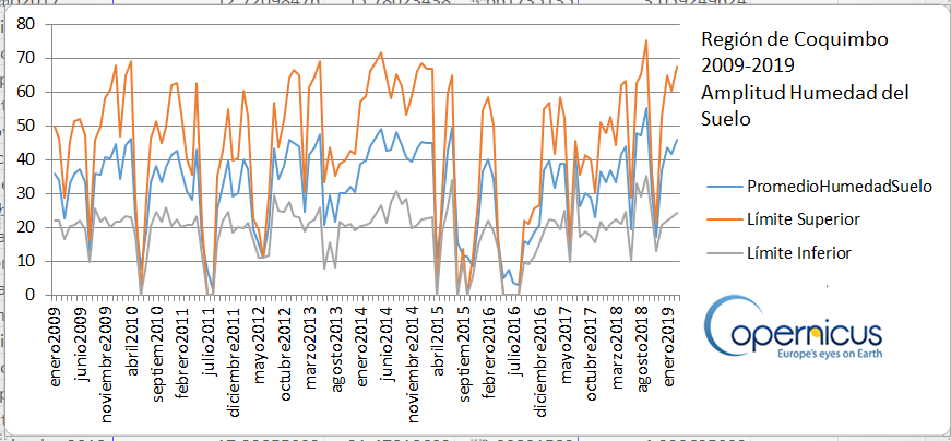
It can be seen that the amplitude is wide in all years. Especially large between the months September 2013 and April 2015. This means that the region shown on the map can be segmented into several parts to have a more uniform data breadth. It would seek to have the idea of low humidity in the rainy season and the most important thing is sunny days for solar radiation in the months of October to April to contribute to the Winkler parameter.
Observe that from October 2018, the amplitude becomes larger which indicates that there are regions that are favoring sunlight, but others have no light to help with the growth of the vine.
4.2) Valparaíso y Roncagua REGIONS
In Valparaíso and Roncagua, the regions studied by satellite are on these maps.
Imagen 4.1.3 | Imagen 4.1.4 |
The amplitude of the data for Valparaíso and Rancagua, show these results.
Imagen 4.1.5 Amplitude Soil Water Index. Blue line average. Upper and Bottom limits. |
The standard deviation to obtain the upper and lower limits show that for the dry season, approximately from October to April-May, there is a larger data amplitude than for the rainy season, June-September. This information indicates that humidity in the summer is quite irregular throughout the studied region. Then there is a need to segment it to investigate which territories are the driest during the summer. This is important because these areas favor more growth and the Wrinkler parameter because they are the driest and probably the brightest.
4.3) Maule REGION
La región de Maule es la siguiente: | |
Imagen 4.1.6 | Imagen 4.1.7 |
The breadth of the data shows the following results
Imagen 4.1.8 Amplitude Soil Water Index. Blue line average. Upper and Bottom limits. |

The Maule region is more humid than Valparaíso and Aconcagua. It shows the same situation as Valparaíso-Aconcagua that the dry season does not show uniform humidity throughout the region. It is necessary to segment it to see where you can have the least moisture in the soil and luminosity so that the growth of the vine has a high Wrinkler index.
4.4) Bío Bío REGION
The Bío Bío region is in these maps:
Imagen 4.1.9 | Imagen 4.1.10 |
The breadth of Bío Bío data is observed here
Imagen 4.1.11 Amplitude Soil Water Index. Blue line average. Upper and Bottom limits. |

What can be deduced from the amplitude and limits is that it is the most regular and uniform region of those that have been studied. Both in the rainy season and in the summer, its standard deviation is small, which means that the upper and lower limits are very close to the average. The clear marking of the seasons of the climate, with heavy rain in winter and quite dry summers, create favorable conditions for the cultivation of the vine. Low soil moisture, which is uniform throughout the region, makes it a destination to consider in order to protect itself from Climate Change.
5) FACTS FROM THE CRISIS OF THE DROUGHT FROM 2009 TO 2018 USING THE COPERNICUS SOIL HUMIDITY INDEX SUPPORTED BY OTHER METEOROLOGICAL AND ECONOMIC INDICATORS
5.1) DROUGHT CRISIS OF CALIFORNIA AND AUSTRALIA MEASURED WITH THE SOIL HUMIDITY INDEX AND MAPS OF THE USA DROUGHT MONITOR UU AND THE OFFICE OF METEOROLOGY OF AUSTRALIA
The drought graph of the Copernicus soil moisture indicator was cross-checked with the US drought monitor maps. UU
(https://droughtmonitor.unl.edu/ ) and the Australian Bureau of Meteorology (http://www.bom.gov.au/climate/ )
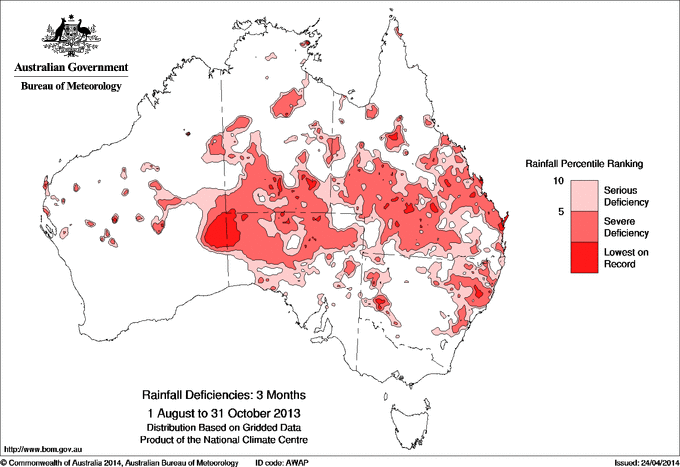
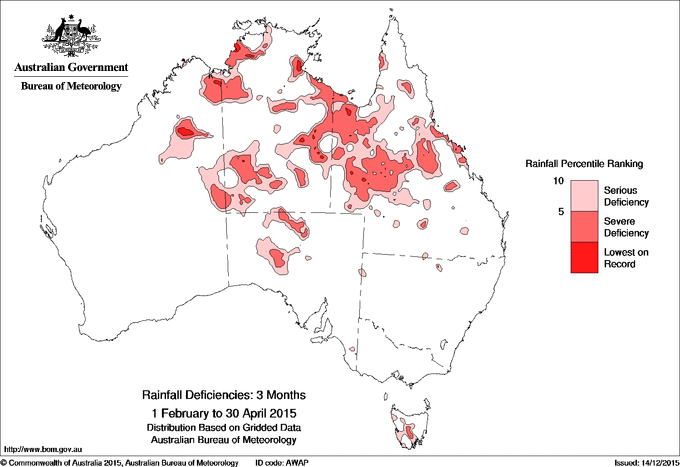
Image 1 shows the Copernicus soil moisture indicator for California and Australia Pacific from 2009 to 2018. The drought crisis can be read and is consistent with other meteorological and economic indicators that are explained below. Also, test the usefulness of the Copernicus Soil Moisture Index for regions such as Central America that do not have expensive sensors to measure in situ drought readings. The data from year to year are:
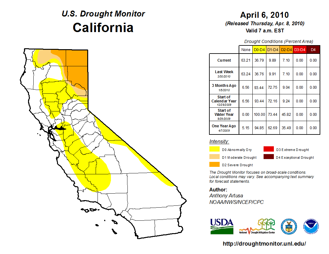
a.1) 2009-2010: Image 1 shows a low soil moisture index in California in 2009. The Map 5, California, map of the US Drought Monitor. UU., Confirms the drought of April 2009. SWI had a slight recovery in California in 2010 confirmed by the map of Image 6 for April 2010. Australia had fallen from SWI in 2010, compared to 2009 (Figure 1).
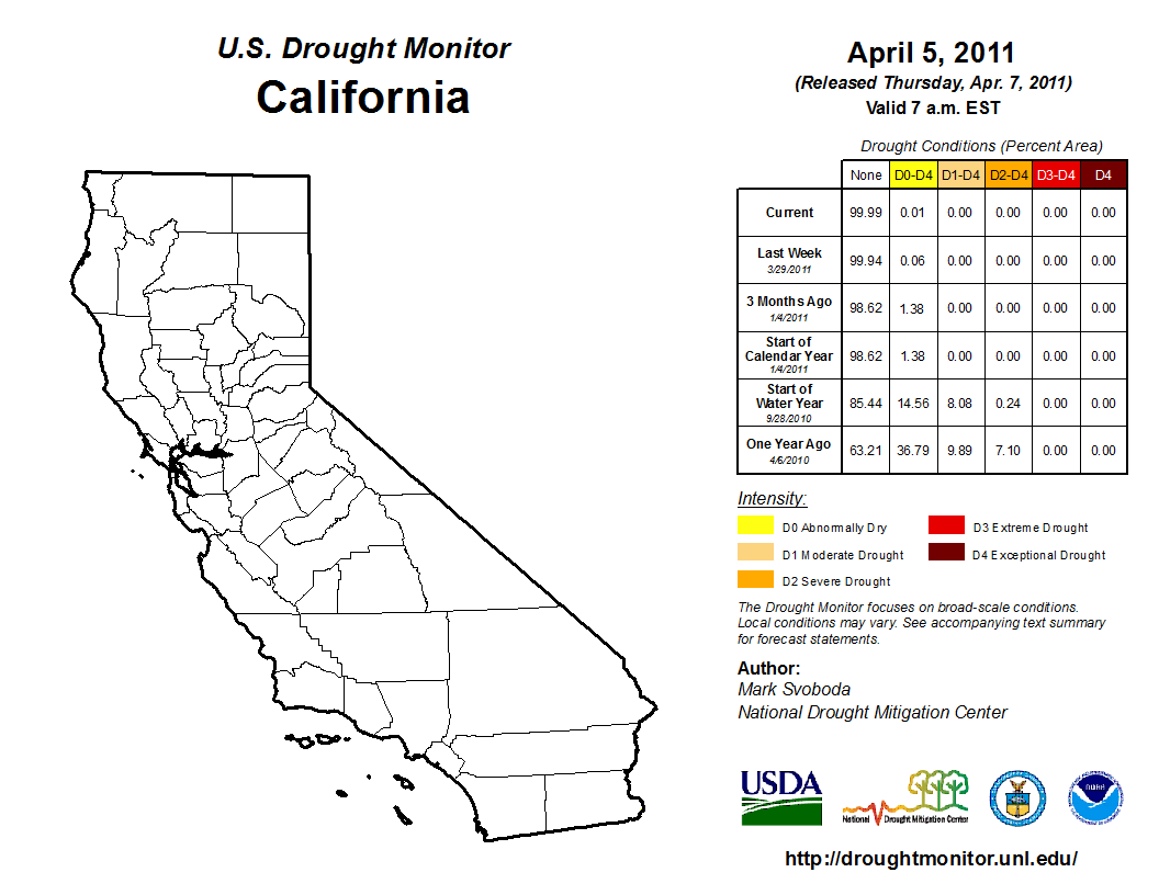
a.2) 2011: California had a fall in the SWI, but the map in Image 7, shows no drought statewide in April 2011. The SWI increase for Australia confirmed by Image 2, the map of the Australian Bureau of Meteorology. After 2011, a five-year drought crisis began.
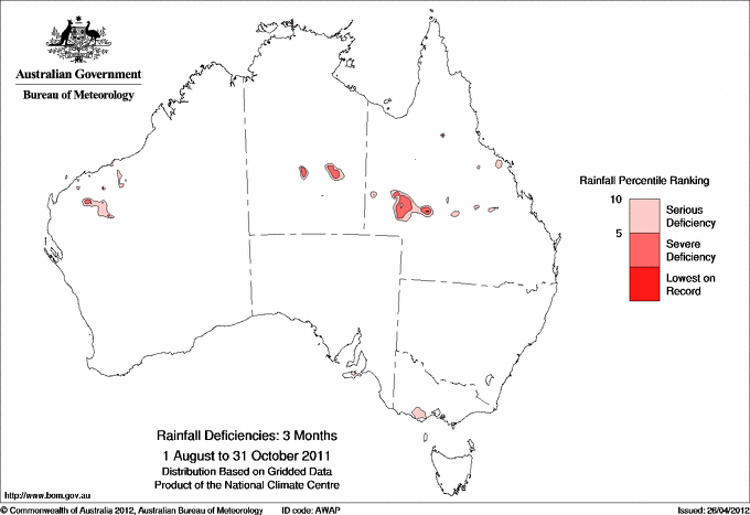
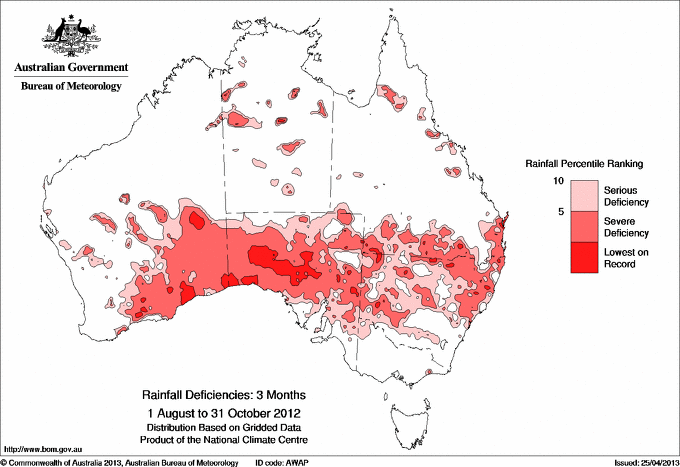
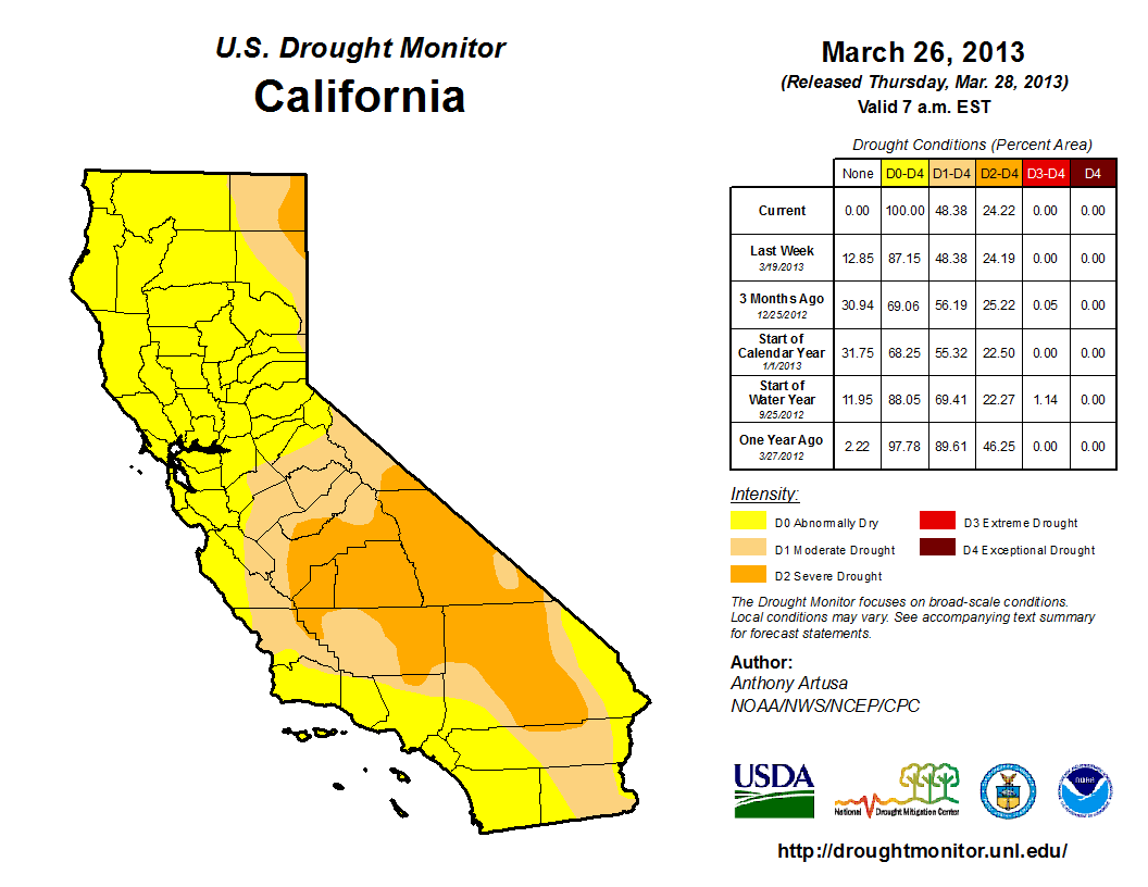
a.3) 2012: SWI for both, California and Australia fell. The signs of drought appear on the maps of both regions in Images 3 (Australia) and 8 (California).
a.4) 2013: The drought continues in California and Australia. SWI low. The maps show the situation.
Images 4, Australia and 9, California.
a.5) 2014: SWI for California had a slight recovery, but not enough to compensate for the years of low rainfall in 2012 and 2013. The map in Figure 10 shows the uncovered moisture deficit. Most of the state suffers a severe drought. Especially the central region: Fresno, Kings, Tulare and Tuolumne.
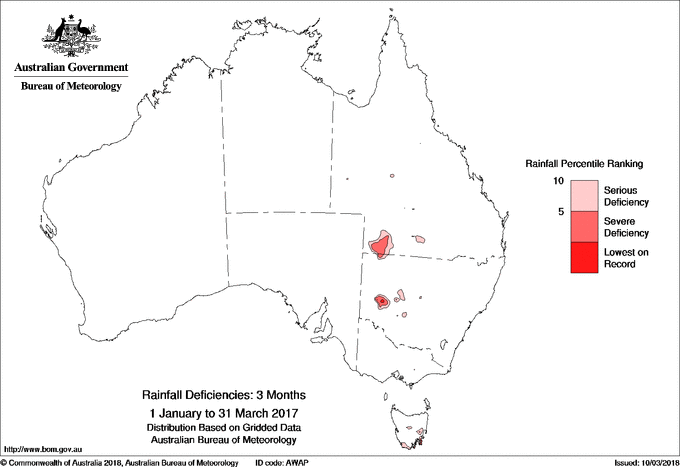
Australia had another year under SWI. The map in Figure 4.1 shows the region of Central Australia affected by the drought. It was the first year of the El Niño event, followed by an extremely dry 2015.
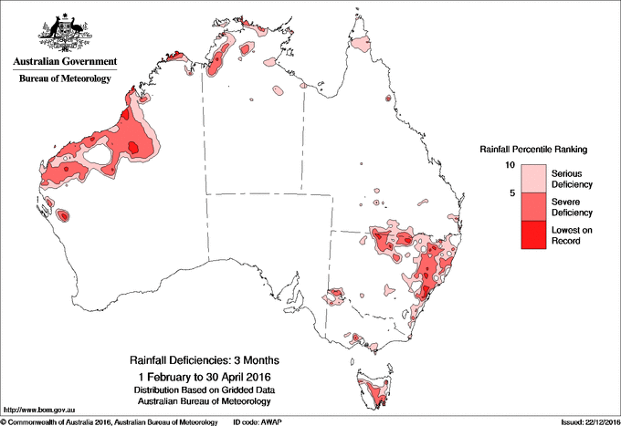
a.6) 2015: The worst year of El Niño since 1998. The SWI for California fell again. Image 11 shows the drought extended to the southern region of the state. The SWI for Australia is low and constant compared to 2014. Image 4.2 shows the drought concentrated in the central and eastern regions of the country.
a.7) 2016: Australia and California had a strong recovery from SWI. Even with this recovery, Figure 12 shows that the drought continues to affect most of the Central Region of the State of California. Image 4.3 indicates that Australia is almost free from drought.
a.8) 2017: Another high SWI indicator for California and Australia compared to 2014 and 2015. Image 13 shows California almost recovered from the drought. Image 14 shows that Australia had no drought this year.
a.9) 2018: Back to the crisis. The SWI for Australia and California shows a severe drop compared to 2017. Image 15 shows the drought again in most of the state. Image 16 shows the southern part of Australia affected by the drought.
References
- USA Drought Monitor (https://droughtmonitor.unl.edu/ ) -Australia Bureau of Meteorology (http://www.bom.gov.au/climate/ )
- California county crops report. Department of Food and Agriculture https://www.cdfa.ca.gov/exec/county/CountyCropReports.html-NOAA : http://www.cpc.ncep.noaa.gov/ - California Department of Water Resources. https://sgma.water.ca.gov/portal/
| ||
Source:USA Drought Monitor | ||
| Image 5.3: August to October 2012. |
|
|
|
|
|
|
|
|
|
|
|
|
|
| Image 5.15: California March 2018 . |
|


5.1.1) IMPACT ON THE ECONOMY IN FRESNO, CALIFORNIA AND UNDERGROUND WATER WELLS
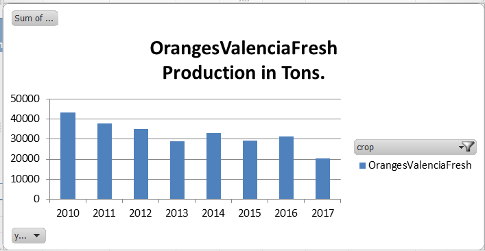
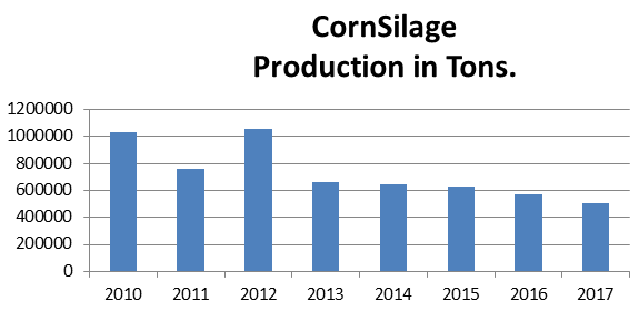
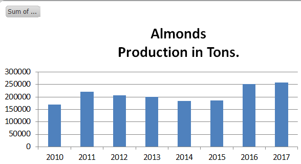
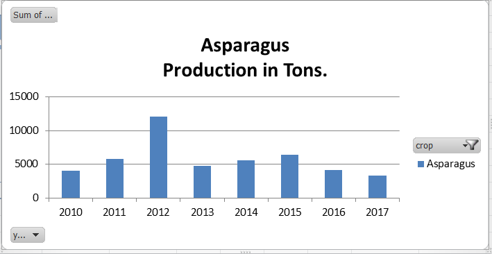
Images 19 to 23 show the production of Valencian oranges, maize silage, almonds, broccoli, and asparagus. As the trend of the Soil Moisture Index for California in Image 1, the production of these products began to fall after 2011-12. With the exception of the almonds that had a recovery for 2016 and 2017, the other products have not yet recovered the levels until 2011.
Image 24 has a sample of ten Fresno Count water wells and their Underground Water Elevation. The levels began to fall after 2013. They had a deep fall after 2016 and have not yet recovered. The California soil water index indicates that the 2018 rainy season fell again, so it has a great effect on the levels of groundwater elevation of the water wells.
Source: California county crops reports. Department of Food and Agriculture. | ||
Image 5.19 |
| Image 5.21 |
| Image 5.23 | |
| ||


5.2) A POSSIBLE RELATIONSHIP BETWEEN DROUGHTS AND THE TEMPERATURE OF THE PACIFIC OCEAN.
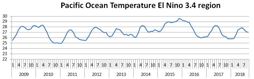
Image 25 shows the temperature of the Pacific Ocean taken from NOAA Equatorial Pacific Sea Surface Temperatures (https://www.ncdc.noaa.gov/teleconnections/enso/indicators/sst/ ). The facts about the El Niño events are: 1) Each year, the temperature rises in June and falls in September. 2) El Niño events cause the temperature to remain high until December. As it happened in 2009-2010. In 2014, the temperature dropped in September but was higher than September levels in previous years. Then it continues to rise throughout 2015. The temperature peak in December 2015 was as high as El Niño in 1982 (Image 26) and 1997 (Image 27). This is probably the reason why these El Niño events have been catastrophic. The temperature in September 2018 fell as expected. But it remains high and equal to 2014. That could explain the evidence of the low water index of the soil for California and Australia in 2018 (Image 1).
Image 5.25 |
Image 5.26 |
Image 5.27 |


5.3) GUATEMALA, CENTRAL AMERICA, THE EFFECTS OF DROUGHT IN HUNGER, IMMIGRATION AND THE LOSS OF COFFEE PRODUCTION
Image 17 indicates the soil water index for three regions of Guatemala.
-The Dry Corridor (Dry Corridor) is an extremely dry region in the eastern part of the country. Like California and Australia, the drought crisis began after 2011 and had a recovery until 2017. These years of drought caused even a lake to disappear, as reported in a National Geographic article (https://news.nationalgeographic.com/2017/05/lake-atescatempa-guatemala-drought-el-nino-video/ ) The rainy season for 2018 has not ended but was already affected by a long dry pause of rain from mid-June to late of August.
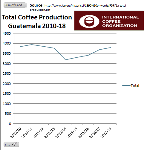
- Coban and Santa Rosa are two coffee producing regions. The fall of the Soil Moisture Index after 2011 created a low production and probably the epidemic of coffee rust that killed several planting areas. The fall of SWI went deeper in 2014-15. The recovery of SWI began after 2016. This crisis caused a drop in coffee production according to statistics from the International Coffee Organization (www.ioc.org ). Image 18 shows the fall in coffee production from 2011 with a serious crisis in 2014. The recovery of production began in 2017. The same year of the increase in the Soil Moisture Index for both coffee producing regions, Coban and Santa Rosa. See Figure 14. The drought in Guatemala and its economic impact caused hunger and a humanitarian crisis due to immigration to the United States. Huffington Post published an article about this situation. Link: https://www.huffingtonpost.com/entry/climate-change-coffee-guatemala_us_589dd223e4b094a129ea4ea2
In 2018, these regions were also affected by a long dry pause of rain from mid-June to the end of August. This is likely to have an effect on coffee production in 2019.
|
Image 5.3.18 |
|
|


6) READING OF SATELLITE DATA OF COPERNICUS WITH PROGRAMMING LANGUAGE "R"
Copernicus uses the NetCDF format (network common data form, https://www.unidata.ucar.edu/software/netcdf/) to generate the satellite data. The NetCDF file consists of several information fields, mainly:
-Latitude
-Length
-Date and reading time
-Data that interests. For example, the Soil Water Index or soil moisture factor that is used in this investigation.
The NetCDF file, read by the SNAP software of the European space agency (http://step.esa.int/main/toolboxes/snap/) consists, for example, of the following fields of information:
Image 6.1 |

The relevant data in this example are:
-Pixel of the north of Chile in Latitude 30 21 S and Longitude 69 57 W.
-Value of Soil Water Index for that point: 93.
-The band used is SWI10. What does it mean reading every 10 days?
6.1) MAIN CODE LINES IN "R" LANGUAGE TO READ THE NETCDF FILE DATA.
The complete code is shown below. It will also be published in GITHUB.
Libraries to use:
library (ncdf4)
library (raster)
library (rgdal)
library (ggplot2)
library (pracma)
File upload NETCDF.
filename <- paste("C:/tempfiles/copernicus/source/",filename01,sep="")
print (filename)
nc_data <- nc_open(filename)
Specify the BAND of data that you want to read. In this case it is the SWI_10, which is the reading of soil moisture every ten days.
ndvi.array <- ncvar_get(nc_data,"SWI_010")
dim (ndvi.array)
Guardarlo en formato RASTER en una variable. Se indica que se desea guardar mínimas y máximas latitudes y longitudes.
r <- raster(t(ndvi.array), xmn=min(lon), xmx=max(lon), ymn=min(lat), ymx=max(lat), crs=CRS("+proj=longlat +ellps=WGS84 +datum=WGS84 +no_defs+ towgs84=0,0,0"))
Code for latitude and longitude ranges to be charged. In this case it is the northern region of Chile. Also specify the date in the ARRAY.
loadata[4,1] <- -29.96 Latitud mayor
loadata[4,2] <- -30.33 Latitud menor
loadata[4,3] <- -70.82 Longitud menor
loadata[4,4] <- -69.96 Longitud mayor
loadata[4,5] <- fecha de carga
loadata[4,6] <- "chile1" Nombre del área a cargar
Cycle to obtain the range of latitudes
for(lati in seq(lati01,lati02,-0.01))
{
Cycle to obtain the range of latitudes
for(longi in seq(longi01,longi02,0.01))
{
Extract spatial data from the Soil Water Index of the desired latitude and longitude
toolik_lon <- longi
toolik_lat <- lati
toolik_series <- extract(r, SpatialPoints(cbind(toolik_lon,toolik_lat)), method='simple')
Convertir en format data_frame los datos espaciales obtenidos arriba
toolik_df <- data.frame(data_swi= seq(from=1, to=1, by=1), SWI_10=t(toolik_series))
Obtener el soil water index asignado a una variable
data_soil_water_index = toolik_df[1,2]
Assign the data set to a variable to be able to write it in a text file separated by commas
queryinsert<-paste(queryinsert,"(", lati,",", longi,",", data_soil_water_index ,",'",
fechadata,"',", "1,'",regiondata ,"')")
Write the data to a text file separated by commas.
outputfile <- paste("C:/tempfiles/copernicus/swiproc/",fechadata,regiondata,".csv")
fileConn<-file(outputfile)
queryinsert<-paste(queryinsert,";")
writeLines(c(queryinsert), fileConn)
close(fileConn)
Complete list of the program in language "R"
#install.packages("pracma")
library (ncdf4)
library (raster)
library (rgdal)
library (ggplot2)
library (pracma)
localuserpassword <- "9Di$icom77"
library(RMariaDB)
EXAMPLE1<-matrix(ncol=300, nrow=300)
filestoload[1,1] <- '2010feb20.nc'
filestoload[1,2] <- '2010-02-20'
filestoload[2,1] <- '2010mar20.nc'
filestoload[2,2] <- '2010-03-20'
filestoload[3,1] <- '2010abr20.nc'
filestoload[3,2] <- '2010-04-20'
filestoload[4,1] <- '2009may20.nc'
filestoload[4,2] <- '2010-05-20'
for (filesloading in 1:1)
{
filename01 <- filestoload[filesloading,1]
fechaload <- filestoload[filesloading,2]
filename <- paste("C:/tempfiles/copernicus/source/",filename01,sep="")
print (filename)
nc_data <- nc_open(filename)
#nc_data <- nc_open('c:/tempfiles/swi20oct2018.nc')
#print (nc_data)
lon <- ncvar_get(nc_data,"lon")
lat <- ncvar_get(nc_data,"lat", verbose = F)
t <- ncvar_get(nc_data,"time")
ndvi.array <- ncvar_get(nc_data,"SWI_010")
dim (ndvi.array)
r <- raster(t(ndvi.array), xmn=min(lon), xmx=max(lon), ymn=min(lat), ymx=max(lat), crs=CRS("+proj=longlat +ellps=WGS84 +datum=WGS84 +no_defs+ towgs84=0,0,0"))
#print (r)
#plot (r)
#r_brick <- brick(r, xmn=min(lat), xmx=max(lat), ymn=min(lon), ymx=max(lon), crs=CRS("+proj=longlat +ellps=WGS84 +datum=WGS84 +no_defs+ towgs84=0,0,0"))
loadata[1,1] <- 15.23
loadata[1,2] <- 12.94
loadata[1,3] <- -90.42
loadata[1,4] <- -87.75
loadata[1,5] <- fechaload
loadata[1,6] <- "guatemala"
loadata[2,1] <- 15.36
loadata[2,2] <- 13.07
loadata[2,3] <- -87.42
loadata[2,4] <- -84.75
loadata[2,5] <- fechaload
loadata[2,6] <- "salhn"
#_____________________________
#Central America North Costa Rica
#_____________________________
loadata[3,1] <- 11.08
loadata[3,2] <- 9.45
loadata[3,3] <- -85.94
loadata[3,4] <- -84.43
loadata[3,5] <- fechaload
loadata[3,6] <- "northcostarica"
#_____________________________
#_____________________________
#Chile
#_____________________________
#_____________________________
#Chile 1
#_____________________________
loadata[4,1] <- -29.96
loadata[4,2] <- -30.33
loadata[4,3] <- -70.82
loadata[4,4] <- -69.96
loadata[4,5] <- fechaload
loadata[4,6] <- "chile1"
#_____________________________
#_____________________________
#Chile 2
#_____________________________
loadata[5,1] <- -32.31
loadata[5,2] <- -34.03
loadata[5,3] <- -71.40
loadata[5,4] <- -70.54
loadata[5,5] <- fechaload
loadata[5,6] <- "chile2"
#_____________________________
#_____________________________
#Chile 3
#_____________________________
loadata[6,1] <- -32.31
loadata[6,2] <- -34.03
loadata[6,3] <- -71.40
loadata[6,4] <- -70.54
loadata[6,5] <- fechaload
loadata[6,6] <- "chile3"
#_____________________________
#_____________________________
#Chile 4
#_____________________________
loadata[7,1] <- -34.01
loadata[7,2] <- -36.11
loadata[7,3] <- -72.37
loadata[7,4] <- -70.33
loadata[7,5] <- fechaload
loadata[7,6] <- "chile4"
#_____________________________
#_____________________________
#Chile 5
#_____________________________
loadata[8,1] <- -35.97
loadata[8,2] <- -38.25
loadata[8,3] <- -72.76
loadata[8,4] <- -71.2
loadata[8,5] <- fechaload
loadata[8,6] <- "chile5"
#_____________________________
for (region in 1:8)
{
lati01 <- loadata[region,1]
#print (lat01)
lati02 <- loadata[region,2]
#print (long01)
longi01 <- loadata[region,3]
#print (lat02)
longi02 <- loadata[region,4]
#print (long02)
fechadata <- loadata[region,5]
regiondata<- loadata[region,6]
countery <- 0
counterx <- 0
indexcounter <- 0
#for(lati in seq(12,19,0.01))
#difference between finish and start
#latitude-longitude multiply by 100 and then
#plus one to get the size of the
#rows-cols for matrix
#This example is for the Guatemala Caribbean
queryinsert<-"INSERT INTO `gibs_temp` (latitud,longitud,temperatura,fecha,tipo,region) VALUES "
for(lati in seq(lati01,lati02,-0.01))
#for(lati in seq(15.23,15.25,0.01))
{
countery <- countery + 1
counterx <- 0
#print(lati)
for(longi in seq(longi01,longi02,0.01))
#for(longi in seq(-89.56,-89.4,0.01))
{
#print(longi)
counterx <- counterx + 1
toolik_lon <- longi
toolik_lat <- lati
toolik_series <- extract(r, SpatialPoints(cbind(toolik_lon,toolik_lat)), method='simple')
toolik_df <- data.frame(data_swi= seq(from=1, to=1, by=1), SWI_10=t(toolik_series))
outputloc <- paste(lati,",",longi,",",toolik_df[1,2],",",fechadata,",",regiondata, "\n")
if (!(is.na(toolik_df[1,2])))
{
if (indexcounter>=1)
{
queryinsert<-paste(queryinsert,",")
}
indexcounter <- indexcounter + 1
queryinsert<-paste(queryinsert,"(",
lati,",",
longi,",",
toolik_df[1,2],",'",
fechadata,"',",
"1,'",
regiondata ,"')")
}
} #END FOR Longi
}#END FOR Lati
outputfile <- paste("C:/tempfiles/copernicus/swiproc/",fechadata,regiondata,".csv")
fileConn<-file(outputfile)
queryinsert<-paste(queryinsert,";")
writeLines(c(queryinsert), fileConn)
close(fileConn)
} #END of region
} #END OF filesloading
6.2) OBTAIN STATISTICAL DATA BY QUERY SQL TO MYSQL DATABASE WITH LANGUAGE "R"
LIBRARY TO USE:
library(RMariaDB)
CONNECTION TO DATABASE TO USE IT AND PERFORM THE QUERY.
storiesDb <- dbConnect(RMariaDB::MariaDB(), user='root', password=localuserpassword, dbname='data_load', host='localhost')
THE QUERY IS BUILT AND THE RESULTS ARE STORED:
sql <- "select distinct(DATE_FORMAT(fecha, '%Y-%m-%d')) from gibs_temp where fecha >= '2010-03-20' and fecha <= '2018-12-20';"
query<-paste(sql)
rs = dbSendQuery(storiesDb,query)
dbRows<-dbFetch(rs)
Loop is created with the number of records obtained from the query:
countOfStories<-nrow(dbRows)
for (i in 1:countOfStories)
{
The desired region is obtained for the date that is processing the loop and the average temperature is obtained:
fechaproc <- dbRows[i,1]
sql <- paste("select avg(temperatura) from gibs_temp where region = ' chile2 ' and fecha = '",fechaproc,"'")
query<-paste(sql)
print(query)
rs01 = dbSendQuery(storiesDb01,query)
dbRows01<-dbFetch(rs01)
results[i] <-dbRows01[1]
The results are written in a file separated by commas, CSV.
dffile.df <- as.data.frame(results)
write.csv(dffile.df, file ="c:/tempfiles/mydata.csv")
Listado completo del código:
localuserpassword <- "password "
library(RMariaDB)
# The connection method below uses a password stored in a variable.
# To use this set localuserpassword="The password of newspaper_search_results_user"
storiesDb <- dbConnect(RMariaDB::MariaDB(), user='root', password=localuserpassword, dbname='data_load', host='localhost')
storiesDb01 <- dbConnect(RMariaDB::MariaDB(), user='root', password=localuserpassword, dbname='data_load', host='localhost')
dbListTables(storiesDb01)
sql <- "select distinct(DATE_FORMAT(fecha, '%Y-%m-%d')) from gibs_temp where fecha >= '2010-03-20' and fecha <= '2018-12-20';"
query<-paste(sql)
rs = dbSendQuery(storiesDb,query)
dbRows<-dbFetch(rs)
countOfStories<-nrow(dbRows)
for (i in 1:countOfStories)
{
fechaproc <- dbRows[i,1]
sql <- paste("select avg(temperatura) from gibs_temp where region = ' northcostarica ' and fecha = '",fechaproc,"'")
query<-paste(sql)
print(query)
rs01 = dbSendQuery(storiesDb01,query)
dbRows01<-dbFetch(rs01)
results[i] <-dbRows01[1]
xvalues <- append(xvalues,i+2)
print (dbRows01[1] )
dbClearResult(rs01)
} #END of FOR countOfStories
dffile.df <- as.data.frame(results)
write.csv(dffile.df, file ="c:/tempfiles/mydata.csv")
dbDisconnect(storiesDb)
dbDisconnect(storiesDb01)
MYSQL data table where soil moisture indexes are stored. In this case, the Soil Water Index is stored in the TEMPERATURE column
CREATE TABLE `gibs_temp` (
`id` int(11) NOT NULL AUTO_INCREMENT,
`latitud` double DEFAULT NULL,
`longitud` double DEFAULT NULL,
`temperatura` double DEFAULT NULL,
`fecha` datetime DEFAULT NULL,
`tipo` int(11) DEFAULT NULL,
`region` varchar(32) DEFAULT NULL,
PRIMARY KEY (`id`),
KEY `latid` (`latitud`) USING BTREE,
KEY `longid` (`longitud`) USING BTREE,
KEY `temper` (`temperatura`) USING BTREE,
KEY `fechadate` (`fecha`) USING BTREE,
KEY `regionestudio` (`region`) USING BTREE
) ENGINE=MyISAM AUTO_INCREMENT=2517039 DEFAULT CHARSET=latin1;